2DKD: a toolkit for content-based local image search

Abstract

Background

Direct comparison of 2D images is computationally inefficient due to the need for translation, rotation, and scaling of the images to evaluate their similarity. In many biological applications, such as digital pathology and cryo-EM, often identifying specific local regions of images is of particular interest. Therefore, finding invariant descriptors that can efficiently retrieve local image patches or subimages becomes necessary.

Results

We present a software package called Two-Dimensional Krawtchouk Descriptors that allows to perform local subimage search in 2D images. The new toolkit uses only a small number of invariant descriptors per image for efficient local image retrieval. This enables querying an image and comparing similar patterns locally across a potentially large database. We show that these descriptors appear to be useful for searching local patterns or small particles in images and demonstrate some test cases that can be helpful for both assembly software developers and their users.

Conclusions

Local image comparison and subimage search can prove cumbersome in both computational complexity and runtime, due to factors such as the rotation, scaling, and translation of the object in question. By using the 2DKD toolkit, relatively few descriptors are developed to describe a given image, and this can be achieved with minimal memory usage.

Background

Moment-based approaches are very useful for representing biological and medical images as they are pixelized [1] or voxelized data [2–4]. In medical imaging, such as computerized tomography (CT) scan and magnetic resonance imaging (MRI), objects are observed at different viewpoints and local images need to be extracted and examined. In digital pathology, for instance, pathologists are interested in information about specific structures rather than the whole image [5]. Thus, it is necessary to construct moment invariants that do not change by translation, rotation, and scaling and can efficiently retrieve local image patches or subimages.

Here we present the software package 2DKD, twodimensional Krawtchouk descriptors, for local comparison of 2D images. The mathematical formulation of 2DKD was already established in [1], which brings in the following advantages: 1) Krawtchouk polynomials are defined on a discrete space, so the moments derived from them do not carry any error due to discretization. 2) These polynomials are orthogonal; each moment extracts a new feature of the image, where minimum redundancy is critical in their discriminative performance. 3) They are complete with a finite number of functions (equal to the image size), while many other polynomial spaces have infinitely many members. 4) They have the ability to retrieve local image patches by only changing the resolution of reconstruction and using low order moments. 5) The location of the patch can also be controlled by changing two parameters and hence shifting the region-of-interest along each dimension [6]. 6) These moments can be transformed into local descriptors, which are invariant under translation, rotation, and scaling [1].

2DKD also has the potential to be used in cryo-electron microscopy imaging (cryo-EM), in particular, single-particle cryo-EM. This method generates a 3D reconstruction of the structure by combining data from many 2D projection images, in which identical copies of a protein complex are found in different orientations [7]. From the images of fields containing a large number of molecular complexes, individual particles need to be selected manually or by automated algorithms for further image processing. In addition to the acquisition of high-quality projection images of the particles, fast and accurate particle selection is also critical to ensure a high-resolution 3D reconstruction of structures [8]. We test the software 2DKD by applying it to particle selection in a 2D projection image of GroEL complexes obtained using cryo-EM.

The recognition accuracy of 2DKD was tested in [1] and compared to the traditional Hu invariants on two different datasets, a dataset of binary images and another one with gray-scale clip art images. The comparisons were made based on the top-ranked hits, where the Euclidean distance was used as the similarity measure between two descriptor vectors. Overall, 2DKD showed better prediction accuracies than Hu invariants. The descriptors in [1] were only tested up to 4% noise. Here, we introduce a more stable version of 2DKD, which shows tolerance up to 30% noise in the image data.

Implementation

Workflow

The workflow of 2DKD software is shown in Fig. 1. For a given query image and the pixel location (x_p,y_p) of a point-of-interest on the image data, 2DKD performs the following six functions.

• 1. readImage: This script reads a standard N×M gray-scale image file and extracts the image as an N×M density function f(x,y).

• 2. prepStep: For the number S (the size of the query image region) determined by readImage or provided by the user, this script computes the 2D central weight function W_c(x,y) corresponding to the parameters p_x=p_y=0.5 (i.e., the center of an S×S image). It also computes the norms ρ(n;p,S−1) and the coefficients a_i,n,p,S−1 corresponding to the Krawtchouk polynomials K_n(x;p,S−1) where n=0,…,3 and i=0,…,n. These initial constants computed in prepStep are for later use, so the rest of the computations is performed on-the-fly. A more detailed description of the weight function can be found in [1].

• 3. squareCrop: This script crops an N×M image density function f(x,y) to a perfect S×S square image data f_s(x,y). The user-supplied point-of-interest location (x_p,y_p) in the input image is updated to its relative location (x_s,y_s) in the square image.

• 4. compDesc: This script translates the central weight function W_c(x,y) to the region of interest within the S×S square grid as needed. If the local point of interest is located at (x_s,y_s), then the new weight is defined by W_s(x,y)=W_c(x^∗,y^∗) with x^∗=x−(S−1)/2+x_s and y^∗=y−(S−1)/2+y_s. Whenever (x^∗,y^∗) is situated outside the grid, we set W_s(x,y)=0. The function is defined on the discrete domain {0,1,…,S−1}×{0,1,…,S−1}. Then using the square S×S image data f_s(x,y) containing the point (x_s,y_s), this script first computes the auxiliary (weighted) image

  $$ \tilde{f}(x,y) = f_{s}(x,y)\cdot W_{s}(x,y), $$

  (1)

  Fig. 1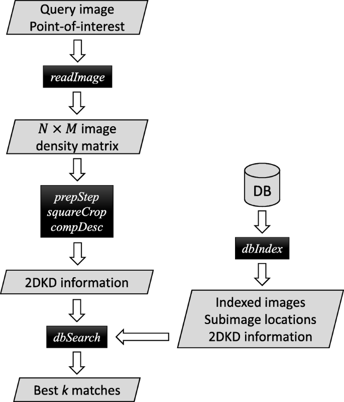

  

  Flow chart of 2DKD. The script names are shown in black boxes

  its geometric moments $\tilde {\mathrm {M}}_{00}$, $\tilde {\mathrm {M}}_{10}$, and $\tilde {\mathrm {M}}_{01}$, the center of mass $(\tilde {x},\tilde {y})$, and the central moments $\tilde {\mu }_{20}$, $\tilde {\mu }_{02}$, and $\tilde {\mu }_{11}$ of $\tilde {f}(x,y)$. It then finds the unique angle $\tilde {\theta }$ between the principal axis of the auxiliary image $\tilde {f}(x,y)$ and the x-axis of the 2D plane. This angle is critical for building the rotation invariant descriptors. The exact computation of $\tilde {\theta }$ is provided in [9]. Using $\tilde {\mathrm {M}}_{00}$, $\tilde {x}$, $\tilde {y}$, and $\tilde {\theta }$, this script calculates the geometric invariants $\tilde {\lambda }_{ij}$ for i,j=0,1,2,3 using the formula provided in [1]. We finally compute the 2DKD using

  $$ \begin{aligned} \tilde{Q}_{nm} &= \left[\rho(n;0.5,S-1)\cdot \rho(m;0.5,S-1)\right]^{-1/2}\\ &\cdot \sum_{i=0}^{n}\sum_{j=0}^{m}a_{i,n,0.5,S-1}\cdot a_{j,m,0.5,S-1}\cdot \tilde{\lambda}_{ij} \end{aligned} $$

  (2)

  for n,m=0,1,2,3 and p_x=p_y=0.5. The descriptors $\tilde {Q}_{00}$, $\tilde {Q}_{01}$, $\tilde {Q}_{10}$, and $\tilde {Q}_{11}$ are removed because they take a constant value irrespective of the region-of-interest we are working with. In this work, we use the 2DKD of order up to 3, that is,

$$ V = \left[\tilde{Q}_{20}, \,\tilde{Q}_{02}, \,\tilde{Q}_{12}, \,\tilde{Q}_{21}, \tilde{Q}_{30}, \,\tilde{Q}_{03}\right]. $$

(3)

Usage example:

• % Change directory to the scripts folder

• >> cd scripts;

• % Full path to the sample image file

• >> impath = ‘../Exp1/DB/image1.jpg’;

• % Point-of-interest location

• >> xp = 180; yp = 480;

• % Read the image to an N×M density data

• >> [f, S] = readImage(impath);

• % Compute the constants for later use

• >> const = prepStep(S);

• % Crop the image data to a square S×S data

• >> [fs, xs, ys] = squareCrop(f, xp, yp, S);

• % Compute 2DKD corresponding to (x_p,y_p)

• >> V = compDesc(fs, xs, ys, const)

• % Output (on the command window)

  V = -0.67263229 -0.67450386 0.00022609 0.00020224 0.00043392 0.00037958

• 5. dbIndex: This high-level script is responsible for producing descriptors for all subimages in the database so that a query can be compared with them. It scans each image in the database by computing the 2DKD for each point-of-interest location and saves the descriptors with the image number and the location of the subimage in that image. The result is stored in a potentially large matrix with rows of the form <Image number, x_p, y_p, V> for easy access later when a subimage is queried. Note that unless there is a change in the database, this only needs to be run once offline to save computational time.

• 6. dbSearch: dbSearch is another high-level script and is used to search the output of dbIndex for descriptors similar to the ones corresponding the query. A query image is supplied as input, then compDesc is run on the query, producing descriptors for it, and then the matrix from dbIndex is sorted by Euclidean distance of descriptors to the new ones obtained, giving a ranked list of the most similar regions to the query from all subimages in the database.

Results

In this section, we present some experimental results and evaluate the discriminative power of 2DKD. For each point of interest (x_p,y_p) corresponding to a subimage, we compute and use the feature vector V given in (3). To compare the descriptors for a query with those for subimages in a database, we use the squared Euclidean distance as a similarity measure, namely

$$ d\left(V^{Q},V^{DB}\right) = \sum_{i=1}^{6} \,\left(V_{i}^{Q}-V_{i}^{DB}\right)^{2}. $$

(4)

Experiment I

To construct the first database, we use nine clip art icons that are downloaded from Microsoft Office Online. These images are shown in Fig. 2. They are transformed to 60×60 gray-scale images and placed in the center of a 150×150 frame to be used as queries. The same set of gray-scale images are also used to generate a database. These images are rotated by the angles

$$ \begin{aligned} \phi = & \;0^{\circ}, 30^{\circ}, 60^{\circ}, 90^{\circ}, 120^{\circ}, 150^{\circ}, \\ & \;180^{\circ}, 210^{\circ}, 240^{\circ}, 270^{\circ}, 300^{\circ}, 330^{\circ}, \end{aligned} $$

(5)

Fig. 2

Nine small gray-scale clip art images used as subimages to generate the first image dataset. Image credit: Microsoft Office Online – clip art gallery

and scaled by the factors

$$ \begin{aligned} s = & \;0.8, 0.9, 1.0, \end{aligned} $$

(6)

to obtain a set of 9×12×3=324 subimages. These subimages are randomly placed in 81 positions to form an image of size 600×600. In this experiment, four such images are generated, one of which is shown in Fig. 3.

Fig. 3

An example 600×600 image from the dataset containing gray-scale clip art subimages

We run dbIndex to produce descriptors for all subimages in the database so a query can be compared with them. After computing the norms, coefficients, and the central weight for S=150, dbIndex scans each image in the database by trimming a 150×150 region from the image containing each point-of-interest, computes 2DKD for each corresponding subimage, and saves them with the image number and the location of the subimage in that image.

From Table 1, it is clear that 2DKD correctly matches the query subimage with the subimages in the dataset successfully with 100% accuracy if we consider the top-ranked hit and 93.3% accuracy when we look at the top 5 hits in the dataset.

Table 1 Total hits and misses for 9 queries

We also tested 2DKD for searching for subimages in the salt-and-pepper noise degraded version of the dataset, with noise densities 10%, 20%, and 30%. The results are summarized in Table 2. Considering only top-ranked hits, our descriptors show tolerance up to 30% noise with only one miss. Among top 5 results, it shows 91.1% accuracy with 10% noise, whereas it decreases to 77.8% with 20% noise, and to 71.1% with 30% noise. Three example queries and corresponding top 5 retrievals from the dataset with 30% noise are shown in Fig. 4.

Fig. 4

Example queries and corresponding retrievals from the dataset with 30% noise. For each query subimage, top 5 matches from the dataset are shown

Table 2 Total number of successful retrievals from the salt-and-pepper noise degraded dataset

Experiment II

Next, we test the local search performance of 2DKD on a more realistic problem, particle selection in 2D projection images of cryo-EM. In single-particle cryo-EM, these projection images contain identical copies of a protein complex in different orientations. One such example is GroEL, a molecular chaperonin found in a large number of bacteria [10]. An example projection image of GroEL protein complexes is shown in Fig. 5a. From these images, individual particles need to be selected by hand or by automated algorithms. Once selected, they are sorted based on variations on their structural features. Similar images are then averaged to obtain representative projection views of the complex at much higher signal-to-noise ratios than in the original images (see Figs. 5b and c.) Finally, the 3D Fourier transform is built up from a collection of 2D images spanning a complete range of orientations and used to recover the 3D structure of the complex via inverse Fourier transform (see Fig. 5d) [7]. Thus, selection accuracy and speed in particle selection are highly important to increase the resolution of reconstructed 3D structures.

Fig. 5

a A section of a projection image of GroEL protein complexes in vitreous ice captured using Cryo-EM. b Averaged top view of GroEL. c Averaged side view of GroEL. d An end-on view of the 3D atomic structure of GroEL complex. Image credits – a Vossman, https://commons.wikimedia.org/wiki/File:Cryoem\_groel.jpg, b, c: Electron Microscopy Data Bank (EMD-8750), d: Protein Data Bank (PDB ID: 5W0S)

We run the script, dbIndex, as in Experiment I to produce descriptors for all subimages in a 1024×1024 projection image (a section of which is shown in Fig. 5a) so a query can be compared with them. The image is very noisy, and there are many flat regions or regions inbetween-particles that should not be considered. We compute the local variance of pixel densities of each 40×40 subregion and compare it against the global pixel density variance. The subregion centers corresponding to lower value of local variances are not indexed. This way, we ensure that we keep the regions with high visibility and discard those with undesired particles. Then we compute 2DKD for each of the remaining subimages using S=40 and save them with the (x,y)−coordinates of the subimage center in the global image. The results are stored in a matrix as in Experiment I. Finally, we query one manually detected top-view of GroEL and search similar ones in the entire indexed image using the script dbSearch. The subregions are ranked by the Euclidean distance as in Experiment I, and top 15 hits are demonstrated in Fig. 6. As justified by the figure, most of the retrievals from global image visually match the query except only three of them: the eleventh, thirteenth, and fourteenth. In this experiment, we only search within one image, but the code can be easily adapted to handle a database with multiple projection images.

Fig. 6

An example query of the top view of GroEL and top 15 retrieval results using 2DKD. The pixel size for the local subimages is 40×40. The (x,y) centers of the query and retrieval results in the 1024×1024 global image are provided under each subimage

Table 3 shows the average times taken for computing 2DKD and using them for database indexing and searching. The programs were run 100 times for each task, and the average times were recorded. For each experiment, the programs were tested on a Windows computer with Intel Core i7-8650U processor of 1.90 GHz and 16 GB memory using GNU Octave, version 5.1.0. The table shows that the average time for computing 2DKD of a typical subimage is in the order of 10⁻³, which allows the database indexing to finish in a reasonable amount of time (within a second to under a minute). Assuming that the descriptors were precomputed and stored, the search can be performed in real-time, which makes the software promising for larger datasets.

Table 3 CPU times (seconds) for 2DKD

Conclusions

Searching biological images for local patterns or specific structures can be computationally challenging due to very low signal-to-noise ratio of these images and the limited number of efficient local invariant descriptors available to perform such searches. We developed 2DKD to address these issues and be used for potentially large biological image databases. 2DKD is developed in Octave (open source) and is publicly available at GitHub website. The source codes can be readily applied to image databases in other fields as well.

Availability and requirements

Project name: 2DKD

Project home page: github.com/kiharalab/2DKD

Operating system: Windows 7/10, Linux

Programming language: GNU Octave (version 5.1.0) or MATLAB R2019a (version 9.6.0)

Other requirements: Java (version 8 update 221)

License: GNU General Public License (version 3)

References

Sit A, Kihara D. Comparison of image patches using local moment invariants. IEEE Trans Image Process. 2014; 23(5):2369–79.
Sit A, Shin W-H, Kihara D. Three-dimensional Krawtchouk descriptors for protein local surface shape comparison. Pattern Recog. 2019; 93:534–45.
Sael L, Li B, La D, Fang Y, Ramani K, Rustamov R, Kihara D. Fast protein tertiary structure retrieval based on global surface shape similarity. Proteins Struct Funct Bioinforma. 2008; 72(4):1259–73.
Han X, Sit A, Christoffer C, Chen S, Kihara D. A global map of the protein shape universe. PLoS Comput Biol. 2019; 15(4):e1006969.
Mehta N, Raja’S A, Chaudhary V. Content based sub-image retrieval system for high resolution pathology images using salient interest points. In: 2009 Annual International Conference of the IEEE Engineering in Medicine and Biology Society. IEEE: 2009. p. 3719–22. https://doi.org/10.1109/iembs.2009.5334811.
Yap PT, Paramesran R, Ong SH. Image analysis by Krawtchouk moments. IEEE Trans Image Process. 2003; 12(11):1367–77.
Milne JL, Borgnia MJ, Bartesaghi A, Tran EE, Earl LA, Schauder DM, Lengyel J, Pierson J, Patwardhan A, Subramaniam S. Cryo-electron microscopy–a primer for the non-microscopist. FEBS J. 2013; 280(1):28–45.
Jiang W, Chiu W. Cryoelectron microscopy of icosahedral virus particles. In: Methods in Molecular Biology. Humana Press: 2007. p. 345–363. https://doi.org/10.1007/978-1-59745-294-6_17.
Teague MR. Image analysis via the general theory of moments. JOSA. 1980; 70(8):920–30.
Roh SH, Hryc CF, Jeong HH, Fei X, Jakana J, Lorimer GH, Chiu W. Subunit conformational variation within individual GroEL oligomers resolved by Cryo-EM. Proc Natl Acad Sci. 2017; 114(31):8259–64.
Acknowledgements
The authors would like to thank Charles Christoffer for the help in creating the GitHub repository at Purdue University.
Funding
This work was supported by the National Science Foundation (DMS1614661 and DMS1614777). DK also acknowledges support from the National Institutes of Health (R01GM123055), the National Science Foundation (CMMI1825941) the Purdue Institute for Drug Discovery.
Author information
Authors and Affiliations
Contributions
DK conceptualized the software and contributed to writing the paper. AS conceived the methodology, directed the development of the software, implemented codes for the software, made all the figures and tables, and contributed to writing the paper. JSD wrote the first draft of the manuscript and implemented codes for the software. All authors read, edited, and approved the final manuscript.
Corresponding author
Ethics declarations
Ethics approval and consent to participate
Not applicable.
Consent for publication
Competing interests
The authors declare no competing interest.
Additional information
Publisher’s Note
Springer Nature remains neutral with regard to jurisdictional claims in published maps and institutional affiliations.
Rights and permissions
Open Access This article is distributed under the terms of the Creative Commons Attribution 4.0 International License (http://creativecommons.org/licenses/by/4.0/), which permits unrestricted use, distribution, and reproduction in any medium, provided you give appropriate credit to the original author(s) and the source, provide a link to the Creative Commons license, and indicate if changes were made. The Creative Commons Public Domain Dedication waiver (http://creativecommons.org/publicdomain/zero/1.0/) applies to the data made available in this article, unless otherwise stated.
About this article
Cite this article
DeVille, J.S., Kihara, D. & Sit, A. 2DKD: a toolkit for content-based local image search. Source Code Biol Med 15, 1 (2020). https://doi.org/10.1186/s13029-020-0077-1
Received:
Accepted:
Published:
DOI: https://doi.org/10.1186/s13029-020-0077-1